Jev can see now
October 20, 2026
In the first post I compared three ways to make a decoder LLM choose between options. All three get a probability for each option from a single forward pass over the prompt, without any decoding. Decoding is what happens when you use an LLM as a chatbot or a code assistant. The model predicts one token, appends it to the text and runs again for the next one, until the answer is complete. This loop is the slow part of an LLM, and all three methods avoid it.
This post builds on the third method, the pointer head. The first two methods keep the LM head, the last layer, which maps a latent vector to a probability for every token in the vocabulary. So the options have to be something the model can write. Label logits put a letter A, B or C in front of each option and compare the probabilities of these letters. Sequence likelihood scores the whole written answer, like “The car should stop.” This works well when the options are text. It is awkward when the options are places in an image, because there is no token for “the third object from the left”. You could draw letters onto the image, but then something else has to find the objects first. The pointer head drops the LM head. It compares the latent vector of the question directly with one latent vector for each option, and as we will see, the parts of an image have latent vectors too.
Recap: the pointer head. The prompt contains a question and the options as text:
The traffic light is red. What should the self-driving car do?

Options:
speed up
stop
turn around
One forward pass gives a latent vector at every token. The query is \(h_n\), the vector at the last token of the prompt. It has seen the question and all the options. The key of option \(j\) is \(h_{e_j}\), the vector at the last token of that option (“up”, “stop”, “around”). Two small trained matrices \(W_q, W_k\) project both, and the score is an inner product:
\[s_j = (W_q h_n)^\top (W_k h_{e_j}), \qquad p = \mathrm{softmax}(s).\]The backbone stays frozen. Only \(W_q\) and \(W_k\) are trained, on questions with known answers.
In the first post the options were written out in the prompt, as a list of short answers after the question. A robot usually does not get such a list. It gets a task, like “clear the table”, and a camera feed, and the things it can act on are objects and places in the image. The pointer head only needs one latent vector per option, so it does not matter whether an option is a few words in the prompt or a region of an image. If the image becomes part of the prompt, and each region of it gets its own latent vector, we can use the head from the first post without any change.
Most of this post explains how a vision-language model turns an image into something its language model can read in the same way it reads text. Once the image is in the prompt, pointing at an object in it is done by the same pointer head as before.
I use Qwen again, this time Qwen3-VL-2B, a Qwen that takes images and is small enough for a free Colab GPU. All numbers below come from the notebook.

A vision transformer in a few lines
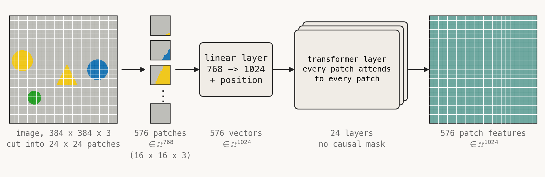
A vision transformer (ViT) is an encoder transformer like BERT, with image patches instead of words. It works in four steps, shown in the figure from left to right.
- Cut the image into patches. A transformer works on a sequence of vectors, one per token. Text comes in discrete tokens, an image does not, so we have to decide what a token is. Single pixels would give 147,456 tokens for a 384 × 384 image, and the cost of attention grows with the square of the sequence length. So the image is cut into non-overlapping patches, and each patch becomes one token. With a patch size of 16 pixels, a 384 × 384 image becomes a 24 × 24 grid, so 576 patches. Each patch, 16 × 16 pixels with three colour channels, is flattened to a vector in \(\mathbb{R}^{768}\) (\(16 \cdot 16 \cdot 3 = 768\)).
- Embed each patch. Image patches are embedded like text tokens, with a learned linear map. For a text token, the input is a one-hot vector as long as the vocabulary, so the map just picks one row of its matrix. That is why it is usually called the embedding table. For a patch, the input is its 768 pixel values, and the map \(W_E: \mathbb{R}^{768} \to \mathbb{R}^{d_v}\), with \(d_v = 1024\), mixes all of them. So patches that look alike get similar vectors, even if the encoder has never seen them before. \(d_v\) is the hidden size of the vision encoder, and every latent vector in every layer of the encoder lives in \(\mathbb{R}^{d_v}\).
-
Add the position. Attention has no built-in sense of order. Every patch is compared with every other patch using the same weights. So if you shuffle the patches, the outputs come out shuffled in the same way, and nothing else changes. Without extra information, the encoder could not tell a patch in the top left from one in the bottom right. There are two common ways to tell each patch its row \(r_i\) and column \(c_i\).
The original ViT adds a learned position vector to each patch embedding. \(P\) is a learned table with one vector per grid cell, and the input to the first layer is
\[x_i = W_E\, \mathrm{patch}_i + P_{r_i, c_i}.\]Rotary position embeddings (RoPE) leave the input alone and act inside every attention layer instead. They split the query and key vectors into pairs of coordinates and rotate each pair by an angle proportional to the position. For the row of patch \(i\) and one pair, with \(R(\phi)\) the 2 × 2 rotation by \(\phi\), the query becomes \(R(\theta r_i)\, q_i\), and the key of patch \(j\) becomes \(R(\theta r_j)\, k_j\). A rotation transposed is the rotation backwards, so the attention score is
\[\big(R(\theta r_i)\, q_i\big)^\top R(\theta r_j)\, k_j = q_i^\top R\big(\theta (r_j - r_i)\big)\, k_j.\]The score depends only on how far apart the two patches are, not on where they are. Each pair of coordinates uses its own \(\theta\), so there are both fast and slow rotations. In 2D, some pairs are rotated by the row and the others by the column.
The encoder in Qwen3-VL uses both. It adds learned absolute embeddings, interpolated to the size of the grid, and it applies 2D RoPE in every layer. Qwen3, the text model, uses only RoPE, over the 1D position in the sequence.
- Run transformer layers without a causal mask. Every patch attends to every other patch. There is no reason for a patch in the top left not to see the bottom right.
The output is one feature vector per patch, so 576 vectors in \(\mathbb{R}^{1024}\). Before the transformer layers, a patch vector only describes its own 16 × 16 pixels. In the figure, a patch on the edge of the yellow circle shows some yellow and some grey table, and a patch on the edge of the yellow triangle looks much the same. After the layers, each of them has attended to the patches around it, and its vector also says what it is part of, a circle or a triangle.
Text transformers do the same with words. In “the bank of the river” and “the bank raised its rates”, the token “bank” starts from the same row of the embedding table. Only after the attention layers have pulled in “river” or “rates” does its latent vector mean a riverbank or a financial institution. A patch vector before the layers is like that first embedding of “bank”. It knows its own pixels and nothing about its surroundings. The main difference to a decoder LLM is the missing causal mask, so every patch gets its context from the whole image, not only from the patches before it.
The vision encoder in Qwen3-VL-2B has 24 layers and about 300M parameters.
Attaching it to a language backbone
Qwen3-VL-2B consists of the vision encoder from above, a small projector, and a Qwen3 language model with 1.7B parameters. The language model is a decoder like the Qwen3-0.6B from the first post. Both have 28 layers, but its latent vectors have \(d = 2048\) dimensions instead of 1024.
Recall what the language model does with text. The tokenizer turns the prompt into token IDs, and the embedding table turns each ID into a vector in \(\mathbb{R}^{d}\). From there on, the 28 layers only work with these vectors. They never see where a vector came from, so any vector in \(\mathbb{R}^{d}\) can take a place in the sequence, also one that does not come from the embedding table. This is how the image gets in.
The vision encoder gives us 576 vectors in \(\mathbb{R}^{d_v}\) with \(d_v = 1024\), but the language model needs vectors in \(\mathbb{R}^{d}\) with \(d = 2048\). So two things are missing. We need a map from the space of the vision encoder into the space of the language model, and we need places for the resulting vectors in the sequence. The projector does the first, and a placeholder in the prompt the second.
The projector. It first combines each 2 × 2 block of neighbouring patches into one vector, by concatenating their four feature vectors into a vector in \(\mathbb{R}^{4 \cdot 1024} = \mathbb{R}^{4096}\). An MLP with one hidden layer, \(\mathbb{R}^{4096} \to \mathbb{R}^{4096} \to \mathbb{R}^{2048}\), then maps it into the space of the language model. The result is 144 vectors in \(\mathbb{R}^{2048}\), one per 32 × 32 pixels of the image. They are usually called image tokens or visual tokens, although they never pass through the tokenizer. I will call them image tokens.
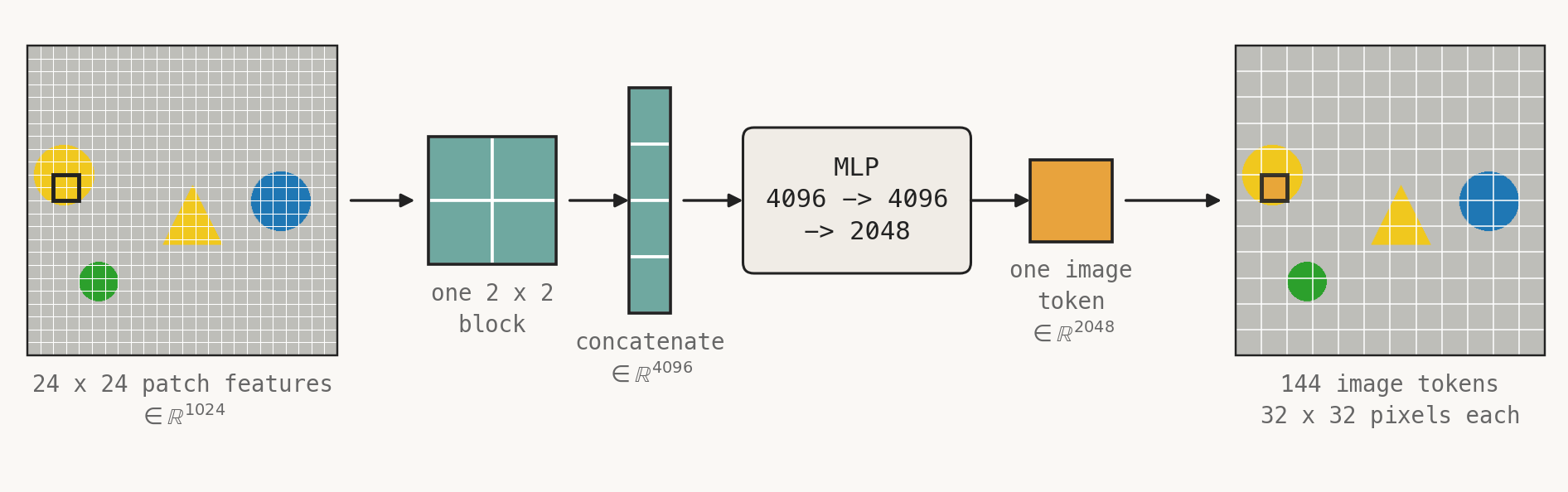
We combine neighbouring patches to save compute. The language model processes every token in each of its 28 layers, and the cost of attention grows with the square of the sequence length, so four times fewer image tokens is a big saving. The price is resolution. The pointer head that we build below cannot point more precisely than one 32 × 32 cell.
Qwen was trained with this 2 × 2 combination, so we cannot easily remove it. All Qwen3-VL models use it, from 2B to 235B parameters, so in each of them one image token covers 32 × 32 pixels. The resolution comes from the size of the input image instead. Qwen3-VL takes images of several megapixels, and a 768 × 768 image would already give 576 image tokens instead of 144. On a real robot I would use a larger image, and probably a larger model. I chose the 2B model and 384 × 384 images so that everything runs on a free Colab GPU, and for our scenes that is enough. The objects are 48 to 88 pixels wide, so each of them still covers a few image tokens.
Making room in the prompt. The tokenizer only handles text, so it cannot put the image into the sequence. Instead, the prompt contains a special placeholder token, <|image_pad|>, where the image goes. This is the prompt for one scene, written out as text:
<|im_start|>user
<|vision_start|><|image_pad|><|vision_end|>Pick up the yellow circle.<|im_end|>
<|im_start|>assistant
<|vision_start|> and <|vision_end|> mark where the image begins and ends, and <|image_pad|> stands for the image tokens. The processor, Qwen’s preprocessing step that prepares the image and the text together, knows that this image gives 144 image tokens. So before tokenizing, it replaces the single <|image_pad|> with 144 copies of it, and the sequence now has 144 slots for the image. The embedding table turns all tokens into vectors as usual, and then the 144 vectors in these slots are replaced by the 144 outputs of the projector.
patches: (576, 1536)     grid: 24 x 24
sequence length: 160     of which image tokens: 144
The image is cut into 24 × 24 = 576 patches with 1536 = 2 · 16 · 16 · 3 values each, because the encoder also handles video and sees a single image as two identical frames. The 2 × 2 combination turns the 576 patches into 144 image tokens, and with the 16 text and markup tokens the sequence has 160.
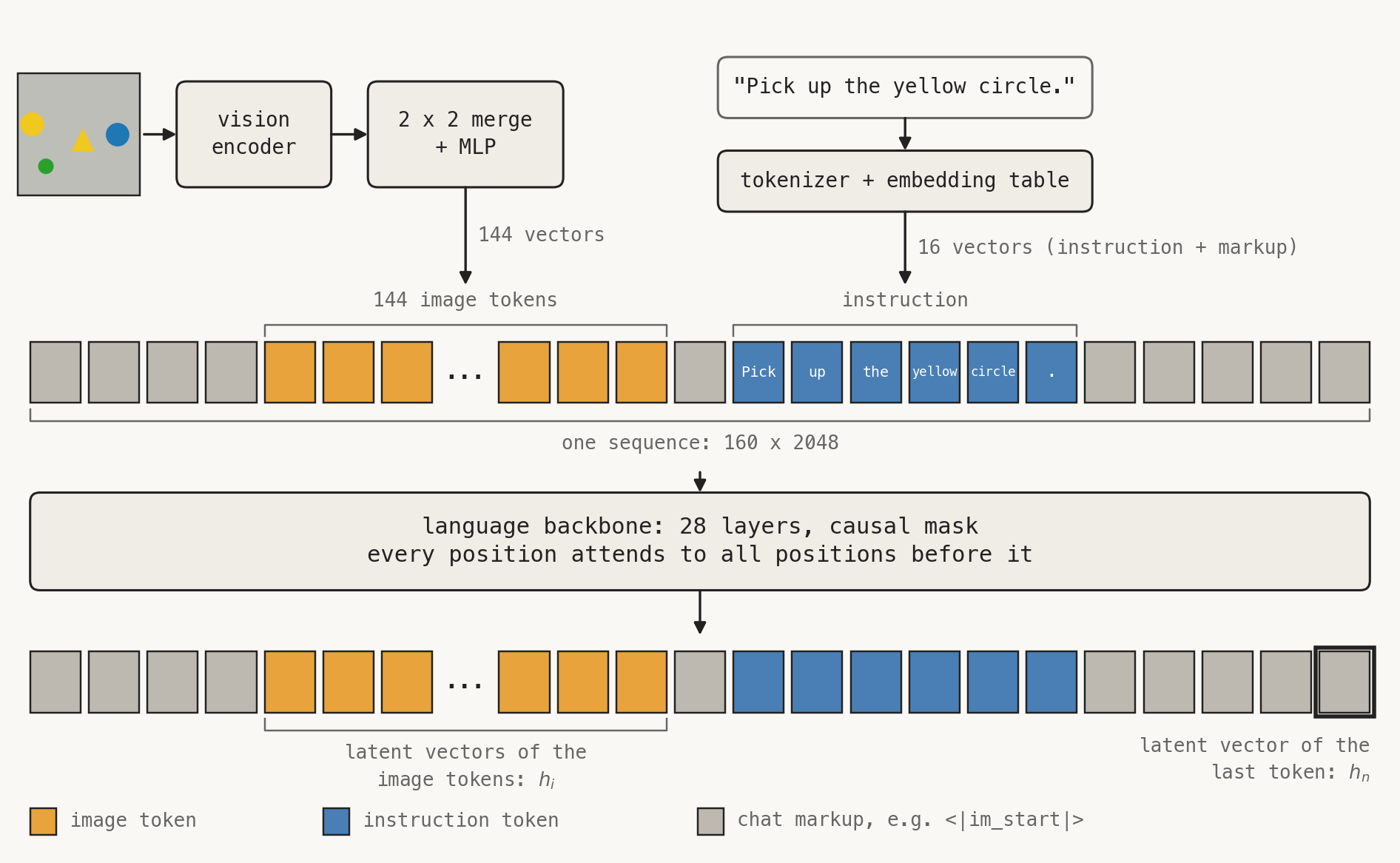
Inside the language model, the image has no extra attention module. Image and text are mixed by the attention layers of the backbone. When the model processes the token “circle”, it attends to the 144 image positions before it in the same way it attends to earlier words. Everything from the first post still applies. There is a latent vector \(h_i\) at every position, including the image positions, and the causal mask runs over the whole sequence.
Two details. The backbone has to know that the 144 image tokens form a 12 × 12 grid and not a line, so Qwen’s position encoding gives each image token its row and its column. And Qwen3-VL has a second, smaller path for the image. It takes features from three intermediate layers of the vision encoder and adds them to the image positions in the first three layers of the language model. I ignore that here, because it changes neither where the image tokens are nor what the pointer head sees.
How does the language model learn to read these vectors? The vision encoder and the language model are pretrained separately. In the simplest recipe, only the projector is trained at first, on image-caption pairs. It has to translate vision features into vectors that make the language model produce the right caption. After that, everything is fine-tuned together.
The task
Pick up the red circle.
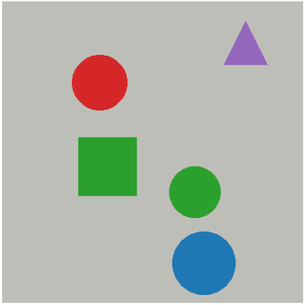
Each scene is a grey table, 384 × 384 pixels, with a few random coloured shapes on it, and an instruction that names one of them. There are six colours and three shapes, circles, squares and triangles, so 18 combinations. Six of them never appear in the training scenes. The test scenes use them to check whether the head reads the instruction or only recognises objects it was trained on. The scene above is one of them, and we come back to it in the results.
Pointing by generating text
Qwen3-VL can already point without any training. If you use it like a chatbot and ask it where the yellow circle is, it writes the answer as text:
<points x1="784" y1="805" alt="yellow circle">yellow circle</points>
The numbers are positions relative to the image, scaled to 0…1000. So x = 0 is the left edge and x = 1000 the right edge, whatever the size of the image in pixels. The target box spans 277 to 336 pixels in x, which is 721 to 875 on that scale, so the point is on the object. On my test scenes, this lands on the right object 93% to 95% of the time.
This is not what we do in this post, but it is the baseline to compare with, and it is the token-intensive way. The answer has 27 tokens, and each token needs its own forward pass, which has to wait for the previous one. In the terms of the first post, this is one prefill and 26 decode steps. For one image that does not matter. For a robot that has to decide several times per second, it does.
The pointer head over image tokens
In the first post the score of option \(j\) was
\[s_j = (W_q h_n)^\top (W_k h_{e_j}),\]with \(h_n\) at the last token of the prompt and \(h_{e_j}\) at the last token of option \(j\). Now every image token is an option. We take the latent vector \(h_i\) at each of the 144 image positions and score it against the same query:
\[s_i = (W_q h_n)^\top (W_k h_i), \qquad p = \mathrm{softmax}(s) \in \mathbb{R}^{144}.\]So there are 144 keys for one query. That is still cheap. The 144 latent vectors come out of the forward pass anyway, and scoring them is one small matrix product, about 75 million multiply-adds next to roughly 300 billion for the forward pass itself.
\(p\) is a probability over places in the image. An object covers several image tokens, so the loss is the negative log of the total probability on the target object \(T\):
\[\mathcal{L} = -\log \sum_{i \in T} p_i.\]Summing \(p\) over the tokens of each object turns it back into Jev-style probabilities over options, where each option is a region of the image.
This is an excerpt from the notebook. Q, K and M are batches of queries, image-token latents and masks of the tokens on the target.
LAYER = 21   # of 28; the last layer works a few points worse, see below

def latents(img, instruction):
    """One pass. Returns h_n (d,) and the latent vectors of the 144 image tokens (144, d)."""
    _, inputs = prepare(img, instruction)
    with torch.no_grad():
        H = model(**inputs, output_hidden_states=True).hidden_states[LAYER][0]
    return H[-1].float().cpu(), H[inputs.input_ids[0] == IMG].cpu()

W_q, W_k = torch.nn.Linear(d, r, bias=False), torch.nn.Linear(d, r, bias=False)
scores = lambda Q, K: torch.einsum("bnr,br->bn", W_k(K.float()), W_q(Q)) / r**0.5   # one score per image token

logp = scores(Q, K).log_softmax(-1)
loss = -torch.logsumexp(logp.masked_fill(~M, -1e9), -1).mean()                      # M: tokens on the target
Two remarks.
The keys do not know the instruction. The image comes before the instruction in the prompt, and the causal mask means an image token only sees what comes before it. So \(h_i\) describes what is at that place in the image, and nothing about what we asked for. Only the query \(h_n\) has seen both. The head matches “what am I looking for” against “what is here”. In the first post I wrote that the question has to come before the options. That was too strong. It lets the options see the question, but the head does not need that. And putting the image first is useful, because its keys and its KV cache can be reused for every new instruction about the same image.
Which layer. I take the latent vectors from layer 21 of 28. The last layer is shaped by its job of predicting the next token, and it gave a few points less here.
Results
The backbone is frozen. The head consists of the two matrices \(W_q, W_k \in \mathbb{R}^{r \times d}\). Here \(d = 2048\) is the latent dimension of the language model, and \(r = 256\) is the dimension of the smaller space in which the query and the keys are compared. That makes \(2rd \approx 1\)M parameters. The head is trained on 800 scenes. A prediction counts as correct if the image token with the highest score lies on the target object. Chance is 26%.
| new scenes, seen combinations | unseen combinations | forward passes | |
|---|---|---|---|
| Pointer head | 96.0% | 85.0% | 1 |
| Generating coordinates as text | 93% | 95% | 27 |
For the text approach, both columns are new to the model, so the difference between 93% and 95% is noise.
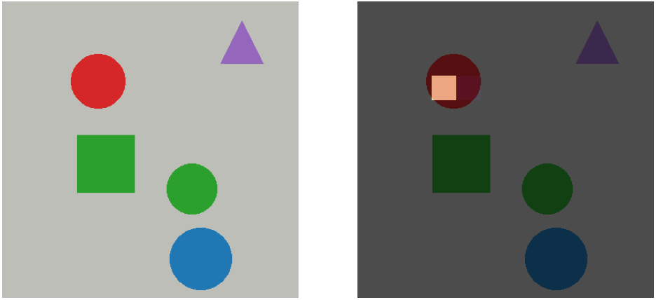
This is the scene from the task section, with the instruction “Pick up the red circle.” On the left is the scene, on the right the probability \(p\) over the 144 image tokens. Red circles never appeared in training. Still, almost all of the probability sits on one image token inside the red circle. The green and the blue circle have the right shape but the wrong colour, and they get nothing. Summed over the tokens of each object, with “table” for all tokens that lie on no object:
blue circle      0.000
purple triangle  0.000
red circle       1.000
green square     0.000
green circle     0.000
table            0.000
The main result is the 85% of the pointer head on unseen combinations. That Qwen generalises well is no surprise, and generating the coordinates as text works very well. But as we saw, it is slow, because it needs 27 forward passes one after the other. In the first post I claimed that a pointer head generalises too, because its trained part contains nothing about any particular option. Here we can see this on a simple, abstract example. The head has never been trained on a red circle, but it has seen red squares and blue circles. It seems that the backbone already encodes colour and shape in both the query and the keys, and the head only has to learn to compare them.
The pointer head is still below the 95% of the text approach. That one comes from a model trained on far more pointing data than my 800 scenes, and the head is hungry for data:
  50 training scenes   seen 32.5%   unseen 30.0%
 100 training scenes   seen 46.0%   unseen 38.5%
 200 training scenes   seen 69.5%   unseen 51.0%
 400 training scenes   seen 79.5%   unseen 67.0%
 800 training scenes   seen 96.0%   unseen 85.0%
The curve is still rising at 800. Scenes are cheap here, so more data is the obvious next step, before LoRA on the backbone.
Is this still Jev?
Only half. Jev makes a decision. It gets a situation and a list of options and picks one. Here the instruction already contains the decision. Nobody had to work out that the yellow circle is the right thing to pick up, the model only has to find it. This is a standard vision-language task called visual grounding. The mechanism is the same as in the first post, though. There is one forward pass, no generated text, and the probability over the options comes from comparing latent vectors.
Doom from the last post would be a real decision task, and it would work in a similar way. Instead of the simple two-dimensional state, the positions of the player and the monster, the prompt would contain the screen image, followed by the options “left”, “right” and “shoot” as text. Then the head is exactly the one from the first post. It scores \(h_n\) against the latent vectors of the option tokens, and the image is context that all of them can attend to. Two things would change. The training data would be screen images labelled with actions, which could be collected automatically, as in the Doom post. And every frame adds 144 or more image tokens to the prompt instead of a few tokens of state, so each step costs more, although it is still a single forward pass. I have not tried that yet. For this post I wanted to focus on the vision part, and pointing at objects shows a different thing that a Jev-style head can do.
Summary
An image enters a language model as a few hundred extra tokens. Each of them has a latent vector, and each belongs to a known place in the image. With a pointer head on these latent vectors, the model can point at an object in a single forward pass, without generating any text. On a frozen backbone, the head is just two small matrices.
This is not new. GUI-Actor decides where to click on a screenshot in the same way, with an attention head between one dedicated token and the image tokens. Most vision-language-action models read their output from the LM head instead, like the first two methods of the first post, which score answer letters or whole written answers. OpenVLA, for example, writes each action as text, one token per action dimension. What I wanted to show is how little is needed to get from the first post to a model that points.