Jev plays Doom
October 08, 2026
We discussed the basics of Jev in the first post about Jev. Let’s now move to a live control loop like a game. I chose Doom because one of the first Jev examples I saw was playing Doom.
To be clear, the real Jev was trained on a big and diverse set of tasks, and we won’t do that here. I have far too little time to curate a good dataset, and the dataset is what makes Jev valuable. The software alone is no moat anymore and there are already several open Jev-like models. This post is about how to use a base LLM for decision making, and specifically how to play a game with an open-weight model like Qwen in a Jev-like way.
I will use a very simple game environment that could also be solved with a logistic regression. But even such a simple game environment shows us some of the issues and possible solutions one might encounter in a more complex scenario.
TL;DR (a very brief technical summary, because today’s post is much more prose than the last one)
- We use a simple state-space environment (only player and monster position) that allows easy data collection (no human-generated data needed). Actions are walk left/right and shoot.
- Zero-shot Qwen (labelling actions with A, B, C in the prompt) does not work.
- A trained pointer head on the player and monster position works slightly better but far from perfect.
- We discovered that Qwen is quite bad at arithmetic. It struggles to get the right move from two positions (monster at 50, player at 100). But it works well if we say monster is 50 to the right.
- We use LoRA to teach Qwen to do the math itself.
A few disclaimers before we start:
We play from the state space, not from the pixel space / video stream. The state is a short vector that describes the situation in the game in compressed form. Here it is two numbers, because we are using a very simple Doom environment (the basic scenario of ViZDoom) where we just have to hit a monster on a shooting range. The only state required here is the sideways position of the player and of the monster, for example:
{'player': 32, 'monster': 52}
Larger numbers are further to the left, so here the monster is 20 units to the left of the player.
That is a very strong simplification. In robotics, getting to such a state is the hard part. A robot has camera images, lidar point clouds, maybe a distance sensor or an AprilTag reading. Nothing tells it “the object is at position 52”, and most of the real work goes into getting from those sensors to a state like this one (even if it is some abstract latent representation). The same holds for games. Playing Doom from the video feed is a much harder task than what we do here. Decisions from pixels are the topic of a later post (coming soon).
We use the simplest Doom scenario and skip reinforcement learning. The training data comes from a hand-written rule, not from an agent that learned to play. More on that below.
So let’s start simple. In the last post we turned a Qwen base model into a classifier over options that are given in the prompt. A game like Doom is a multiple-choice question asked many times per second: here is the situation, here are the actions, pick one. That is what the pointer head from part 1 does. So a small Qwen model with a pointer head should be able to play, with one forward pass per decision and no generated text.
It can, although not out of the box. Here is Qwen3-0.6B playing Doom:
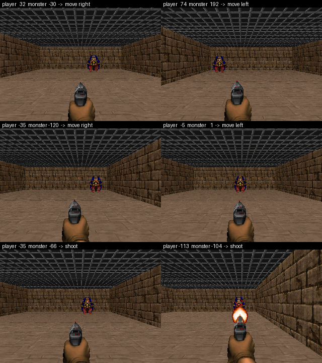
The rest of the post shows how we get there, step by step.

The game
ViZDoom runs Doom as a Python environment. I use its basic scenario: a monster appears somewhere along the opposite wall, and we can move left, move right and shoot. The episode ends when the monster is dead or after 300 tics. The model makes one decision every 4 tics. The reward is +106 for the kill, -5 per shot and -1 per tic, so a good player gets close to +80 and a player that never shoots ends at -300.
The state from above is not computed from the image. The game hands it to us directly:
def read_state(g):
    """The state space: two numbers, the sideways position of the player and of the monster."""
    obj = {o.name: o for o in g.get_state().objects}
    player = round(obj["DoomPlayer"].position_y)
    monster = round(obj["Cacodemon"].position_y) if "Cacodemon" in obj else player   # monster already dying
    return {"player": player, "monster": monster}
Training data from a rule
With the state above, a deterministic rule solves the basic scenario:
def rule(s, tol=24):
    offset = s["monster"] - s["player"]          # > 0: the monster is to the left
    if offset > tol: return 0                    # move left
    if offset < -tol: return 1                   # move right
    return 2                                     # shoot
rule  : reward    79.7   kills 100%   decisions per episode   5.8
random: reward  -124.5   kills  53%   decisions per episode  39.0
The training data is 1500 random states, each labelled with the action the rule takes.
I want to be very clear here: this is an extremely simplified and convenient case to train a policy, which would never occur in real life. The policy is determined by the rule above. So there is really no need to train a complex model, a logistic regression would do it. But for a first toy example, we can take this rule and create training data cheaply. Because, keep in mind, to train the pointer head of our Qwen model, we need training data. And where do we get training data from to train a model on Doom? Either we play several hundred rounds of it ourselves, or we train another reinforcement learning (RL) policy from scratch that learns how to play Doom, and we create training data from that model. Or we could also use “Jev” directly inside the RL loop and train it without producing training data up front.
In a follow-up post we will train another RL policy to create data, and try Qwen directly inside the RL loop.
Qwen, zero-shot
So far the state was a Python dictionary. A language model needs text, so I write the state into a short prompt:
You are playing Doom. You can only move sideways and shoot straight ahead.
Positions are measured along the wall, larger numbers are further to the left.
Your position: 150
Monster position: 43
As a first test I use Qwen without any training, with method 1 from part 1. The three actions are listed in the prompt as A, B and C, and the model is asked to answer with a single letter. We do not let it generate the answer. We read the logits of the three letters and pick the largest.
accuracy: 0.44
how often it picks each action: {'move left': 150, 'move right': 0, 'shoot': 0}
plays: reward  -300.0   kills   0%   decisions per episode  75.0
It answers “A” for every one of the 150 test states. The 44% is the share of states where moving left happens to be right. This is the letter preference from part 1, and a model that only walks left never kills anything.
Pointer head on the frozen backbone
Next is method 3 from part 1, the pointer head. A short reminder of how it works: the three actions go into the prompt as options, one per line and without letters. After one forward pass we take the latent vector at the last token of the prompt, which is the query, and the latent vector at the last token of each option. Two small matrices \(W_q\) and \(W_k\) project them into a common space, and the score of an option is the inner product of its projection with the projection of the query. Here \(W_q\) and \(W_k\) are trained to pick the action of the rule. The backbone is frozen. The order of the options is shuffled for every example, otherwise the head can learn “the answer is the third line” instead of reading the options.
step    0   loss 6.027   test accuracy 0.357
step  500   loss 0.504   test accuracy 0.813
step 2000   loss 0.333   test accuracy 0.827
plays: reward   -17.8   kills  77%   decisions per episode  22.8
83% accuracy, and it plays badly: on average it needs 23 decisions per episode instead of 6, and it fails to kill the monster in 23% of the episodes. The accuracy is stuck between 81% and 83% from step 500 on.
The reason is what the head is asked to do. The action depends on monster - player, compared with a threshold. The head can only combine the latent vectors of the frozen backbone with an inner product. If the backbone has not already computed something like the difference of the two numbers, the head cannot get it out. Apparently a frozen 0.6B model does not lay out the difference between “150” and “43” in a form that an inner product can read.
Doing the subtraction for it
To test that explanation, do the subtraction in Python and write the result into the prompt. The head and the training stay the same.
You are playing Doom. You can only move sideways and shoot straight ahead.
The monster is 107 units to your right.
step    0   loss 5.433   test accuracy 0.393
step  500   loss 0.000   test accuracy 1.000
plays: reward    79.7   kills 100%   decisions per episode   5.8
100%, and it plays like the rule. Reading “to your right” and pointing at “move right” is something a language model is good at. The arithmetic was the problem.
LoRA: letting the backbone learn the arithmetic
Back to the raw coordinates. Instead of doing the arithmetic for the backbone, we let the backbone learn it.
So far the backbone was frozen. All 600M weights of Qwen stayed as they came, and only the pointer head was trained. If the backbone should learn to compare two numbers, its weights have to change. Training all of them is expensive, and with 1500 examples we would mostly damage what the model already knows. LoRA (low-rank adaptation) is a way to change the backbone a little, with very few trainable parameters.
The idea. Take one weight matrix \(W \in \mathbb{R}^{d_\text{out} \times d_\text{in}}\) of the backbone. Fine-tuning changes it to \(W + \Delta W\), where \(\Delta W\) is a full matrix with \(d_\text{out} \cdot d_\text{in}\) entries. LoRA assumes that the change we need is simple, in the sense that \(\Delta W\) has low rank. It writes \(\Delta W\) as a product of two thin matrices:
\[W' = W + \frac{\alpha}{k}\, B A, \qquad B \in \mathbb{R}^{d_\text{out} \times k},\; A \in \mathbb{R}^{k \times d_\text{in}},\; k \ll d.\]\(W\) stays frozen. Only \(A\) and \(B\) are trained. For a \(1024 \times 1024\) matrix and \(k = 8\), that is 16k trainable numbers instead of 1M.
\(B\) starts at zero, so at the beginning \(W' = W\) and training starts exactly at the pretrained model. \(\alpha\) is just a scaling factor. After training, \(BA\) can be added into \(W\) once, so the adapted model is exactly as fast as the original.
Which \(W\)? Every transformer layer has an attention block, and attention uses four weight matrices. Each token computes a query with \(W_Q\) (what am I looking for?) and a key with \(W_K\) (what do I have to offer?). The inner product of query and key decides how much one token attends to another. \(W_V\) then decides what information is passed along, and \(W_O\) writes the result back. It is the same mechanism as the pointer head, which is where its \(W_q\) and \(W_k\) got their names.
I put LoRA on \(W_Q\) and \(W_V\) in each of the 28 layers, which is the usual choice. In Qwen3-0.6B, \(W_Q\) is a \(2048 \times 1024\) matrix and \(W_V\) is \(1024 \times 1024\). Each of these 56 matrices gets its own \(A\) and \(B\).
Why \(W_Q\) and \(W_V\)? It is an empirical result that became a convention, not a law.
- Where it comes from: the original LoRA paper tried different choices for the same parameter budget. Adapting the query and value matrices together did as well as adapting all four attention matrices, and clearly better than putting the whole budget into a single one. Libraries then made “query and value” their default.
- A plausible reason for skipping \(W_K\): attention only ever uses the product of a query and a key. To change which token looks at which, it is enough to change one side of that product, so adapting both is partly redundant.
- Why \(W_V\): it controls a different thing, namely what information is moved once a token is attended to. So query plus value covers “where to look” and “what to bring back”.
- It is not always the best choice. Later work (QLoRA) found that you get closer to full fine-tuning by putting LoRA on every weight matrix, including the MLP blocks. Query and value is the cheap classic setting, and it was enough here.
What the extra term does. A weight matrix is a transformation: it takes a vector \(x\) and returns \(Wx\). With LoRA the layer returns
\[W'x = Wx + \frac{\alpha}{k}\, B\,(Ax).\]The first term is what the pretrained model did anyway. The second term is new, and it works in two steps. \(Ax\) is a vector of only \(k\) numbers. Each row of \(A\) is a direction in the input space, and its number says how much of that direction is in \(x\). Then \(B\) turns these \(k\) numbers into an output vector. Each column of \(B\) is a direction in the output space, and it is added with the weight of its number. So \(A\) decides what to read from the input, and \(B\) decides what to write to the output for it, \(k\) times.
For \(W_Q\) this has a simple meaning. The attention score between token \(i\) and token \(j\) is the inner product of the query of \(i\) with the key of \(j\). With LoRA on \(W_Q\) it becomes
\[\big(W_Q h_i + \tfrac{\alpha}{k} B A h_i\big)^\top W_K h_j = \underbrace{(W_Q h_i)^\top W_K h_j}_{\text{old score}} + \tfrac{\alpha}{k}\, (B A h_i)^\top W_K h_j.\]Every token gets a second query on top of its original one, and every attention score gets an additive correction. The keys stay as they are, so there are no higher-order terms. In our case the token of the monster position could learn an extra query that matches the key of the token of the player position. That is what I would expect it to learn, I did not check what the adapters actually learned.
For \(W_V\) it is the same idea one step later. The value \(W_V h_j\) is what token \(j\) hands over when another token attends to it. With LoRA it hands over \(W_V h_j + \tfrac{\alpha}{k} B A h_j\): \(A\) reads \(k\) features from the token, and \(B\) writes them into the value. The attention pattern decides who talks to whom, and \(W_V\) decides what is said.
With \(k = 8\) and \(\alpha = 16\) this gives 56 adapted matrices and 1.1M trainable parameters, 0.19% of the model. They are trained together with the pointer head. As far as I can tell, this is the setup that Jev-style models use.
epoch 1   test accuracy 0.807
epoch 2   test accuracy 0.947
epoch 3   test accuracy 0.953
epoch 4   test accuracy 0.963
plays: reward    76.8   kills 100%   decisions per episode   6.5
The backbone can learn to compare the two numbers. This is the model in the video at the top.
What this shows
| accuracy | reward | kills | trained parameters | |
|---|---|---|---|---|
| Rule (the expert) | 79.7 | 100% | 0 | |
| Qwen, zero-shot letters | 44% | -300.0 | 0% | 0 |
| Qwen, pointer head, raw numbers | 82.7% | -17.8 | 77% | 0.5M |
| Qwen, pointer head, offset as text | 100% | 79.7 | 100% | 0.5M |
| Qwen, LoRA + pointer head, raw numbers | 96.3% | 76.8 | 100% | 1.7M |
Qwen with LoRA and a pointer head plays this scenario from raw coordinates and kills the monster every time. That is expected. I picked this environment because it is easy, and with the state given, what is left to learn is a function of two numbers.
What I did not expect is how much depended on the way I wrote down the state. The same head got 83% or 100%, depending on whether the prompt said “150 and 43” or “107 to your right”, and I needed LoRA to make the raw numbers work. It is possible that Qwen was not trained on many spatial reasoning tasks (or arithmetic) and therefore is not very good at this.
In the next post I drop the hand-written rule, move to a harder scenario and put Qwen inside an RL loop.